The simplest example of an anisotropic PSF is to consider just a square photosite aperture, without any lens aperture diffraction.
 |
| Figure 1: Edge orientation relative to photosite aperture |
 |
| Figure 2: Fraction of square photosite covered by slanted edge as a function of edge distance to photosite centre |
What can we learn from these curves? Well, we can see that an edge orientation of 45 degrees will overlap with the photosite square from -√0.5 to √0.5, whereas the 0 degrees edge orientation only results in overlap between -0.5 and 0.5. From this we can infer that the square appears wider when approached by an edge with a 45 degree orientation. We also know that a square photosite acts as a low-pass filter, in the sense that the image captured by our sensor is the convolution of this low-pass filter and the analytical model of our scene. This might lead one to believe that the 45 degree case would result in a stronger low-pass filter, because it is clearly "wider" than the 0 degree case.
We can plot the derivative of the curves from Figure 2:
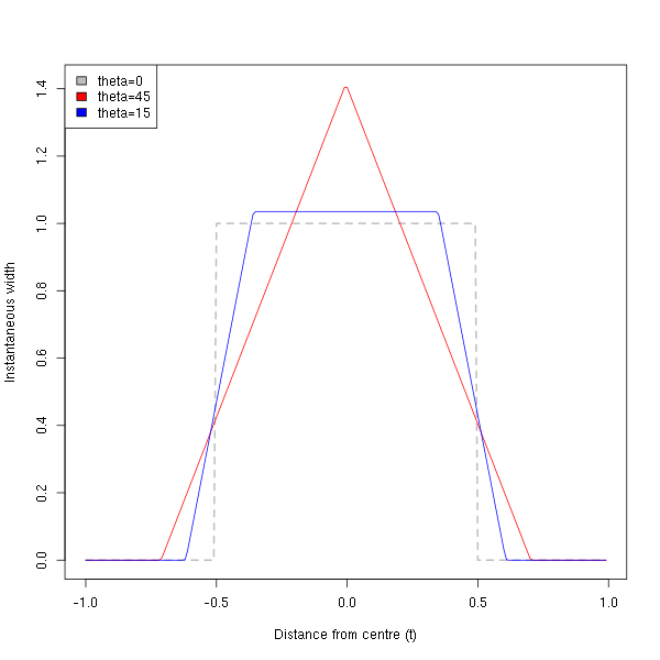 |
| Figure 3: Instantaneous width of PSF |
The 0 degree case is easy to visualize with the help of the left panel of Figure 1: clearly, the width of the photosite square (measured along the step edge) is constant. The 45 degree case is also readily visualized by noting that the we cross the widest part of the photosite square when t=0 (right panel of Figure 1); this nicely corresponds to the peak instantaneous width of √2 in Figure 3.
We can interpret the curve in Figure 3 as a weighting function, i.e., the relative contribution to the convolution of the edge and the photosite aperture at distance t from the centre of the photosite aperture. Looking at the problem this way reveals a new angle: the 45 degree case presents a fair amount of its total weight located close to t=0. Roughly 50.6% of its weight is located in the part where it is wider than the 0 degree case, corresponding to the central of Figure 3 where the red curve is above the gray curve. In contrast, only about 8.6% of the weight of the 45 degree curve is located in the two tail ends (t < -0.5 and t > 0.5). If we compare this to the 0 degree case, we obtain 42% in the centre (area under gray curve where the red curve is above the gray curve), and of course 0% in the tails.
This is a rather unexpected turn of events, since it implies that even though the 45 degree case starts overlapping with the edge sooner (the regions -√0.5 < t < -0.5 and 0.5 < t < √0.5), it represents only a small fraction of the total interaction with the edge. Instead of the 45 degree case being a stronger low-pass filter than the 0 degree case, we expect the opposite because the 45 degree case has roughly 20% (50.6/42) more of its weight located close to t=0.
We appear to have two mildly conflicting views:
a) the 45 degree case is "wider" at its widest point, thus it should be a stronger low-pass filter than the 0 degree case, and
b) more of the weight of the 45 degree case is close to the centre, hence it should present a weaker low-pass filter than the 0 degree case.
I am betting on outcome b), mostly because I already know what the empirical results will tell us ....
Empirical results for square photosites (no diffraction)
The prediction favoured by outcome b) in the previous section tells us that we should expect MTF50 values to increase as we progress from a relative edge orientation of 0 degrees through to 45 degrees. Simulations were performed in the absence of noise, using 30 repetitions over sub-pixel shifts. Keep in mind that the MTF50 value of a square photosite aperture is about 0.6033 cycles per pixel, which is quite high. |
| Figure 4: Square (box) PSF relative MFT50 error as function of edge orientation |
Just to check, let us examine an isotropic PSF: a pure Gaussian without any photosite aperture simulation. This should yield a purely Gaussian MTF. Same simulation, but with the radially symmetric Gaussian PSF:
 |
| Figure 5: Gaussian PSF relative MTF50 error as a function of edge orientation |
Somewhat real world: squares plus diffraction
We have seen that a box PSF (without diffraction) produces strong anisotropy, and that a Gaussian PSF (without photosite aperture) produces no noticeable anisotropy. Using a PSF consisting of an Airy pattern convolved with a square photosite aperture should put us somewhere in the middle of the anisotropy scale.Simulations were repeated using a simulated aperture at f/2.8, light at 550 nm, a photosite pitch of 4.73 micron and no AA (OLPF) filter. These settings give an expected MTF50 value of ~ 0.504 cycles per pixel, which is slightly lower than the expected MTF50 value of ~ 0.6 cycles per pixel seen in the previous section. Accordingly, the MTF50 errors may be slightly reduced (or at least the expected variance should be reduced).
 |
| Figure 6: Airy+box PSF relative MTF50 error as a function of edge orientation |
The trend is clearly visible, but appears to be only about 60% of the magnitude of the case without diffraction (about 2.5% at 44 degrees, vs about 4% without diffraction). Smaller apertures (larger f-numbers) will reduce the anisotropy as the Airy component of the PSF will start to dominate the photosite aperture PSF.
Any practical implications?
The effect of PSF anisotropy on MTF measurements is real, but appears to be relatively small. At 2.5%, do we even have to worry about it?Unfortunately, we have to at least be aware of this for certain types of testing and measurement. Because the error (overestimation) is systematic, it will show up in any measurement that sweeps through a range of angles, just like the MTF Mapper grid test chart, pictured here:
 |
| MTF Mapper grid test chart |
I simulated this chart using mtf_generate_rectangle, using an aperture of f/4, an Airy+box PSF, green light and a photosite pitch of 4.73 micron. Passing this synthetic image through MTF mapper to produce a surface plot (-s option) produces this result:
 |
| Figure 7: MTF50 plot obtained from simulated rendering of the MTF Mapper grid test chart using the Airy-box MTF with a square photosite aperture |
The systematic distortion of MTF50 values is clearly visible, even though the range of values is quite small. The maximum value on the scale is 0.47, which is only about 2% higher than the expected MTF50 value of 0.46073 (at 0 degrees, of course). But the cross pattern is clearly visible. At least I have confirmed the cause.
Pushing for even greater realism I repeated the simulation using the "rounded-square" photosite aperture that MTF Mapper provides. Here is the surface plot:
 |
| Figure 8: MTF50 plot obtained from simulated rendering of the MTF Mapper grid test chart using the Airy-box MTF with a rounded-square photosite aperture |
Lastly, if we use a circular photosite aperture, we get this:
 |
| Figure 9: MTF50 plot obtained from simulated rendering of the MTF Mapper grid test chart using the Airy-box MTF with a circular photosite aperture |
Conclusion
Anisotropy is a reality that we have to deal with if we apply the slanted edge method to edges that approach a relative orientation of 45 degrees with respect to the (presumed) square photosites. The isotropy of the Airy pattern helps to attenuate the overestimation of edges approaching 45 degrees, but the systematic effect is still clearly visible in simulated images.I tried to construct an elegant analytical explanation for the interaction between the edge orientation and a square photosite aperture. This turned out to be harder than I expected, so I only have some interesting plots to offer for now. What did emerge from the theory is that we should not focus on the apparent width of the photosite aperture, but rather on the distribution of its weight relative to the centre. The somewhat startling conclusion is that we should observe higher MTF50 measurements when the orientation approaches 45 degrees.
This was supported by the actual experiments using simulated imagery.
So what can we do about this systematic distortion? Well, the only sound solution would be to stick to edges with a relative orientation of about 5 degrees. This is not a universal solution, though, because it makes it impossible to measure in the true Sagittal/Meridional directions. Imatest solved the problem by sticking to 5 degree angles and referring to "horizontal" and "vertical" MTF. This works well enough if you wish to measure peak astigmatism, but it does not allow you to measure MTF in the optically more appropriate sagittal/meridional directions.
I might add a 5-degree test chart to MTF Mapper in future, just to cover all bases.
No comments:
Post a Comment